TwoBody.jl

TwoBody.jl: A Julia package for solving quantum-mechanical two-body problems

TwoBody.jl provides a flexible framework for constructing two-body Hamiltonians and solving the corresponding Schrödinger equation using a variety of numerical methods. It covers approaches ranging from basis-set and grid methods to tensor-network, stochastic, and neural-network methods. Beyond serving as a proof of concept for FewBody.jl, TwoBody.jl is designed to support practical, cross-scale calculations of quantum two-body systems, from hadrons to molecules.

Install

Run the following command in the Julia REPL or a notebook:

import Pkg; Pkg.add("TwoBody")

Usage

Run the following code before each use.

using TwoBody

Define the Hamiltoninan. This is an example for the non-relativistic Hamiltonian of hydrogen atom in atomic units:

\[\hat{H} = - \frac{1}{2} \nabla^2 - \frac{1}{r}\]

H = Hamiltonian(
  Kinetic(hbar = 1, m = 1),
  Coulomb(coefficient = -1),
)

The usage depends on the method. Define the basis set for the Rayleigh-Ritz Method:

\[\begin{aligned} \phi_1(r) &= \exp(-13.00773 ~r^2), \\ \phi_2(r) &= \exp(-1.962079 ~r^2), \\ \phi_3(r) &= \exp(-0.444529 ~r^2), \\ \phi_4(r) &= \exp(-0.1219492 ~r^2). \end{aligned}\]

BS = BasisSet(
  SimpleGaussianBasis(13.00773),
  SimpleGaussianBasis(1.962079),
  SimpleGaussianBasis(0.444529),
  SimpleGaussianBasis(0.1219492),
)

You should find

\[E_{n=1} = -0.499278~E_\mathrm{h},\]

which is amazingly good for only four basis functions according to Thijssen(2007). The exact ground-state energy is $-0.5~E_\mathrm{h}$.

julia> solve(H, BS)# method

Rayleigh-Ritz method with SimpleGaussianBasis{Float64}
J. Thijssen, Computational Physics 2nd Edition (2013)
https://doi.org/10.1017/CBO9781139171397

# basis function

φ₁(r) = TwoBody.φ(SimpleGaussianBasis{Float64}(a=13.00773), r)
φ₂(r) = TwoBody.φ(SimpleGaussianBasis{Float64}(a=1.962079), r)
φ₃(r) = TwoBody.φ(SimpleGaussianBasis{Float64}(a=0.444529), r)
φ₄(r) = TwoBody.φ(SimpleGaussianBasis{Float64}(a=0.1219492), r)

# eigenfunction

ψ₁(r) = + 0.096102φ₁(r) + 0.163017φ₂(r) + 0.185587φ₃(r) + 0.073701φ₄(r)
ψ₂(r) = + 0.119454φ₁(r) + 0.081329φ₂(r) + 0.496216φ₃(r) - 0.205916φ₄(r)
ψ₃(r) = - 0.010362φ₁(r) + 1.744891φ₂(r) - 0.629196φ₃(r) + 0.097774φ₄(r)
ψ₄(r) = - 6.155100φ₁(r) + 1.240202φ₂(r) - 0.226412φ₃(r) + 0.030780φ₄(r)

# eigenvalue

E₁ = -0.4992784056674876
E₂ = 0.11321392045798988
E₃ = 2.592299571959808
E₄ = 21.144365190122507

# verification

n 	norm, <ψₙ|ψₙ> = cₙ' * S * cₙ = 1
1	1.0
2	1.0000000000000004
3	1.0
4	0.9999999999999988

n 	ill-conditioned, |<ψₙ|H|ψₙ> - E| = |cₙ' * H * cₙ - E| = 0
1	1.8318679906315083e-15
2	3.4833247397614286e-15
3	3.552713678800501e-15
4	1.7763568394002505e-14

# expectation value

n 	hamiltonian, <ψₙ|H|ψₙ> = cₙ' * H * cₙ
1	-0.49927840566748577
2	0.1132139204579864
3	2.5922995719598116
4	21.14436519012249

n 	expectation value of Kinetic(hbar=1, m=1)
1	0.4992783686700055
2	0.8428088332141158
3	4.432656608731446
4	26.465623640332108

n 	expectation value of Coulomb(coefficient=-1)
1	-0.9985567743374912
2	-0.7295949127561295
3	-1.8403570367716344
4	-5.321258450209621

The wave function is also good. However, the Gaussian basis does not satisfy the Kato’s cusp condition.

# solve
res = solve(H, BS)

# benchmark
import Antique
HA = Antique.HydrogenAtom(Z=1, Eₕ=1.0, a₀=1.0, mₑ=1.0, ℏ=1.0)

# plot
using CairoMakie
fig = Figure(size=(420,300), fontsize=11, backgroundcolor=:transparent)
axis = Axis(fig[1,1], xlabel=L"$r / a_0$", ylabel=L"$\psi(r) / a_0^{-3/2}$", ylabelsize=16.5, xlabelsize=16.5, limits=(0,4,0,1.1/sqrt(π)))
lines!(axis, 0..5, r -> abs(TwoBody.ψ(res,r)), label="TwoBody.jl")
lines!(axis, 0..5, r -> abs(Antique.wavefunction(HA, r, 0, 0)), linestyle=:dash, color=:black, label="Antique.jl")
axislegend(axis, position=:rt, framevisible=false)
fig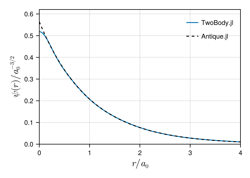

Hydrogen atom benchmark

The following table compares the two lowest $s$-wave energies of the hydrogen atom in atomic units. Here $n=0$ denotes the ground state and $n=1$ the first excited state. The numerical values use the example settings from the corresponding method pages: 20 Gaussian functions for RR, the nine-function complement basis ($M_n=9$) for FC, $\Delta r=0.1$ and $r_\mathrm{max}=50$ for FDM, the default 1024-point grid ($\mathtt{quantics}=10$) for QTT+DMRG, and the documented training or sampling settings for VNN and VMC. A dash indicates that the state is not currently available.

Method	$n=0$	$n=1$
RR	-0.499981735104	-0.124997703473
FC	-0.499999999978	-0.123665583532
FDM	-0.498756211209	-0.124921972504
QTT+DMRG	-0.499702911360	-0.124981415403
VNN	-0.468779111883	—
VMC	-0.480218518855	—
Exact	-0.500000000000	-0.125000000000

TwoBody.jl

Install

Usage

Hydrogen atom benchmark

API reference