Rayleigh-Ritz Method
This method is one of the variational method. It solves the generalized eigenvalue problem,
\[\pmb{H} \pmb{c} = E \pmb{S} \pmb{c}.\]
The Hamiltonian matrix is defined as $H_{ij} = \langle \phi_{i} | \hat{H} | \phi_{j} \rangle$ and the overlap matrix is defined as $S_{ij} = \langle \phi_{i} | \phi_{j} \rangle$. The eigenvector $\pmb{c}$ is the column of the optimal coefficients $c_i$ for the linear combination,
\[\psi(r) = \sum_i c_i \phi_i(r),\]
to minmize the expectation value of the energy,
\[E = \frac{\langle\psi|\hat{H}|\psi\rangle}{\langle\psi|\psi\rangle}.\]
Note that the nonlinear parameters (e.g., exponents of the Gaussian basis functions) are not optimized. The expectation by trial wavefunction is the upper bound for the exact energy.
Theory
In the Rayleigh-Ritz method, the trial wave function is written as a linear combination of basis functions $\phi_1, \phi_2, \phi_3, \ldots$:
\[\psi = \sum_i c_i \phi_i.\]
We then seek the expansion coefficients $c_i$ that minimize the energy $E[\psi]$. The coefficients are ultimately obtained by solving the generalized eigenvalue problem
\[\boldsymbol{H}\boldsymbol{c} = E\boldsymbol{S}\boldsymbol{c}.\]
The derivation is given below. First, let us define the notation. $\boldsymbol{H}$ is the Hamiltonian matrix, whose elements are
\[H_{ij} = \langle \phi_i | \hat{H} | \phi_j \rangle,\]
and $\boldsymbol{S}$ is the overlap matrix, whose elements are
\[S_{ij} = \langle \phi_i | \phi_j \rangle.\]
Substituting $\psi = \sum_i c_i \phi_i$ into $E[\psi]$ gives
\[\begin{aligned} E[\psi] &= \frac{\langle \psi | \hat{H} | \psi \rangle} {\langle \psi | \psi \rangle} \\ &= \frac{\left\langle \sum_i c_i \phi_i \middle| \hat{H} \middle| \sum_j c_j \phi_j \right\rangle} {\left\langle \sum_i c_i \phi_i \middle| \sum_j c_j \phi_j \right\rangle} \\ &= \frac{\sum_{i,j} c_i c_j \langle \phi_i | \hat{H} | \phi_j \rangle} {\sum_{i,j} c_i c_j \langle \phi_i | \phi_j \rangle} \\ &= \frac{\sum_{i,j} c_i c_j H_{ij}} {\sum_{i,j} c_i c_j S_{ij}}. \end{aligned}\]
Here and below, the basis functions and coefficients are assumed to be real. For a complex-valued basis, the coefficient on the bra side must be replaced by its complex conjugate $c_i^*$. The expansion above follows directly from the distributive law and can be seen explicitly by writing $\sum_i c_i \phi_i = c_1 \phi_1 + c_2 \phi_2 + \cdots$.
We minimize this expression subject to the normalization constraint
\[\sum_{i,j} c_i c_j S_{ij} = 1.\]
Using the method of Lagrange multipliers, define
\[L(c_i,E) = \sum_{i,j} c_i c_j H_{ij} - E \sum_{i,j} c_i c_j S_{ij} + E.\]
When $L$ is differentiated with respect to $c_k$, only terms for which $i=k$ or $j=k$ remain. Therefore,
\[\begin{aligned} \frac{\partial L}{\partial c_k} &= 0, \\ \sum_i c_i H_{ik} + \sum_j c_j H_{kj} - E \sum_i c_i S_{ik} - E \sum_j c_j S_{kj} &= 0, \\ 2 \sum_j H_{kj} c_j - 2E \sum_j S_{kj} c_j &= 0, \\ \sum_j \left(H_{kj}c_j - E S_{kj}c_j\right) &= 0, \\ \boldsymbol{H}\boldsymbol{c} - E\boldsymbol{S}\boldsymbol{c} &= 0, \\ \boldsymbol{H}\boldsymbol{c} &= E\boldsymbol{S}\boldsymbol{c}. \end{aligned}\]
In the third line, we used $H_{ij}=H_{ji}$ and $S_{ij}=S_{ji}$, which hold for the real-valued case considered here. Similar derivations can be found in the following references:
- J. M. Thijssen, Computational Physics (Japanese translation, Maruzen Publishing, 2012), Sec. 3.1, Variational Calculations.
- A. Szabo and N. S. Ostlund, Modern Quantum Chemistry: Introduction to Advanced Electronic Structure Theory, Vol. 1 (Japanese translation, University of Tokyo Press, 1987), Sec. 1.3.2, The Linear Variational Problem.
In Julia, the generalized eigenvalue problem $\boldsymbol{H}\boldsymbol{c} = E\boldsymbol{S}\boldsymbol{c}$ can be solved easily with the LinearAlgebra standard library:
using LinearAlgebra
E, c = eigen(H, S)
It is therefore not necessary to know the details of the eigensolver here. The practical challenge is instead to evaluate the matrix elements $H_{ij} = \langle \phi_i | \hat{H} | \phi_j \rangle$ and $S_{ij} = \langle \phi_i | \phi_j \rangle$, and to choose basis functions for which these elements can be calculated efficiently.
Usage
Run the following code before each use.
using TwoBodyDefine the Hamiltoninan. This is an example for the non-relativistic Hamiltonian of hydrogen atom in atomic units:
\[\hat{H} = - \frac{1}{2} \nabla^2 - \frac{1}{r}\]
H = Hamiltonian(
  Kinetic(hbar = 1, m = 1),
  Coulomb(coefficient = -1),
)
Define the basis set:
\[\begin{aligned} \phi_1(r) &= \exp(-13.00773 ~r^2), \\ \phi_2(r) &= \exp(-1.962079 ~r^2), \\ \phi_3(r) &= \exp(-0.444529 ~r^2), \\ \phi_4(r) &= \exp(-0.1219492 ~r^2). \end{aligned}\]
BS = BasisSet(
  SimpleGaussianBasis(13.00773),
  SimpleGaussianBasis(1.962079),
  SimpleGaussianBasis(0.444529),
  SimpleGaussianBasis(0.1219492),
)
Solve the eigenvalue problem. You should find
\[E_{n=1} = -0.499278~E_\mathrm{h},\]
which is amazingly good for only four basis functions according to Thijssen(2007). The exact ground-state energy is $-0.5~E_\mathrm{h}$.
julia> solve(H, BS)# method

Rayleigh-Ritz method with SimpleGaussianBasis{Float64}
J. Thijssen, Computational Physics 2nd Edition (2013)
https://doi.org/10.1017/CBO9781139171397

# basis function

φ₁(r) = TwoBody.φ(SimpleGaussianBasis{Float64}(a=13.00773), r)
φ₂(r) = TwoBody.φ(SimpleGaussianBasis{Float64}(a=1.962079), r)
φ₃(r) = TwoBody.φ(SimpleGaussianBasis{Float64}(a=0.444529), r)
φ₄(r) = TwoBody.φ(SimpleGaussianBasis{Float64}(a=0.1219492), r)

# eigenfunction

ψ₁(r) = + 0.096102φ₁(r) + 0.163017φ₂(r) + 0.185587φ₃(r) + 0.073701φ₄(r)
ψ₂(r) = + 0.119454φ₁(r) + 0.081329φ₂(r) + 0.496216φ₃(r) - 0.205916φ₄(r)
ψ₃(r) = - 0.010362φ₁(r) + 1.744891φ₂(r) - 0.629196φ₃(r) + 0.097774φ₄(r)
ψ₄(r) = - 6.155100φ₁(r) + 1.240202φ₂(r) - 0.226412φ₃(r) + 0.030780φ₄(r)

# eigenvalue

E₁ = -0.4992784056674876
E₂ = 0.11321392045798988
E₃ = 2.592299571959808
E₄ = 21.144365190122507

# verification

n 	norm, <ψₙ|ψₙ> = cₙ' * S * cₙ = 1
1	1.0
2	1.0000000000000004
3	1.0
4	0.9999999999999988

n 	ill-conditioned, |<ψₙ|H|ψₙ> - E| = |cₙ' * H * cₙ - E| = 0
1	1.8318679906315083e-15
2	3.4833247397614286e-15
3	3.552713678800501e-15
4	1.7763568394002505e-14

# expectation value

n 	hamiltonian, <ψₙ|H|ψₙ> = cₙ' * H * cₙ
1	-0.49927840566748577
2	0.1132139204579864
3	2.5922995719598116
4	21.14436519012249

n 	expectation value of Kinetic(hbar=1, m=1)
1	0.4992783686700055
2	0.8428088332141158
3	4.432656608731446
4	26.465623640332108

n 	expectation value of Coulomb(coefficient=-1)
1	-0.9985567743374912
2	-0.7295949127561295
3	-1.8403570367716344
4	-5.321258450209621
Example of Hydrogen Atom
Analytical solutions are implemented in Antique.jl.
# solve
using TwoBody
H = Hamiltonian(Kinetic(1, 1), Coulomb(-1))
BS = GeometricBasisSet(SimpleGaussianBasis, 0.1, 80.0, 20)
res = solve(H, BS)

# benchmark
import Antique
HA = Antique.HydrogenAtom(Z=1, Eₕ=1.0, a₀=1.0, mₑ=1.0, ℏ=1.0)

# energy
using Printf
println("Total Energy Eₙ")
println("------------------------------")
println(" n     numerical    analytical")
println("------------------------------")
for n in 1:4
  @printf("%2d  %+.9f  %+.9f\n", n, res.E[n], Antique.energy(HA; n=n))
end

# wave function
using CairoMakie
fig = Figure(
  size = (840,600),
  fontsize = 11,
  backgroundcolor = :transparent
)
for n in 1:4
  axis = Axis(
    fig[div(n-1,2)+1,rem(n-1,2)+1],
    xlabel = L"$r~/~a_0$",
    ylabel = L"$4\pi r^2|\psi(r)|^2~ /~{a_0}^{-1}$",
    xlabelsize = 16.5,
    ylabelsize = 16.5,
    limits=(
      0, [5, 15, 30, 50][n],
      0, [0.6, 0.2, 0.11, 0.07][n],
    )
  )
  lines!(axis, 0..50, r -> 4π * r^2 * abs(TwoBody.ψ(res,r,n=n))^2, label="TwoBody.jl")
  lines!(axis, 0..50, r -> 4π * r^2 * abs(Antique.wavefunction(HA, r, 0, 0; n=n))^2, label="Antique.jl", color=:black, linestyle=:dash)
  axislegend(axis, "n = $n", position=:rt, framevisible=false)
end
fig
Total Energy Eₙ
------------------------------
n numerical analytical
------------------------------
1 -0.499981735 -0.500000000
2 -0.124997703 -0.125000000
3 -0.055554578 -0.055555556
4 -0.031249107 -0.031250000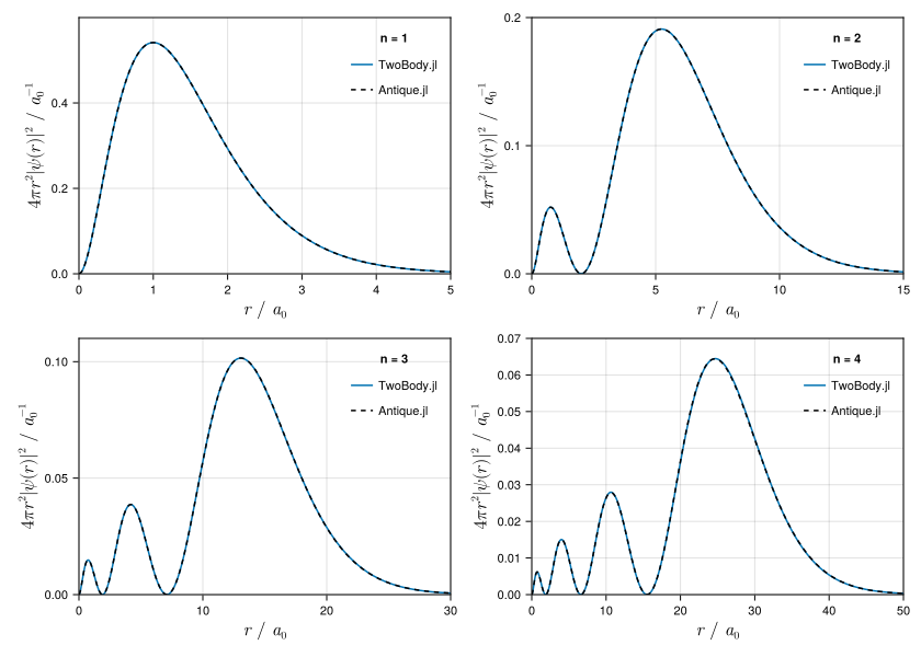
Example of Spherical Oscillator
Analytical solutions are implemented in spherical oscillator.
# solve
using TwoBody
H = Hamiltonian(Kinetic(1, 1), PowerLaw(coefficient=1/2, exponent=2))
BS = GeometricBasisSet(SimpleGaussianBasis, 1.0, 10.0, 20)
res = solve(H, BS)

# benchmark
import Antique
SO = Antique.SphericalOscillator(k=1.0, μ=1.0, ℏ=1.0)

# energy
using Printf
println("Total Energy Eₙ")
println("------------------------------")
println(" n     numerical    analytical")
println("------------------------------")
for n in 1:4
  @printf("%2d  %+.9f  %+.9f\n", n-1, res.E[n], Antique.energy(SO; n=n-1))
end

# wave function
using CairoMakie
fig = Figure(
  size = (840,600),
  fontsize = 11,
  backgroundcolor = :transparent
)
for n in 1:4
  axis = Axis(
    fig[div(n-1,2)+1,rem(n-1,2)+1],
    xlabel = L"$r~/~a_0$",
    ylabel = L"$4\pi r^2|\psi(r)|^2~ /~{a_0}^{-1}$",
    xlabelsize = 16.5,
    ylabelsize = 16.5,
    limits=(
      0, [4.5, 5.0, 5.5, 6.0][n],
      0, [0.90, 0.75, 0.70, 0.65][n],
    )
  )
  lines!(axis, 0..50, r -> 4π * r^2 * abs(TwoBody.ψ(res,r,n=n))^2, label="TwoBody.jl")
  lines!(axis, 0..50, r -> 4π * r^2 * abs(Antique.wavefunction(SO, r, 0, 0; n=n-1))^2, label="Antique.jl", color=:black, linestyle=:dash)
  axislegend(axis, "n = $(n-1)", position=:rt, framevisible=false)
end
fig
Total Energy Eₙ
------------------------------
n numerical analytical
------------------------------
0 +1.500000000 +1.500000000
1 +3.500000001 +3.500000000
2 +5.500000002 +5.500000000
3 +7.500005422 +7.500000000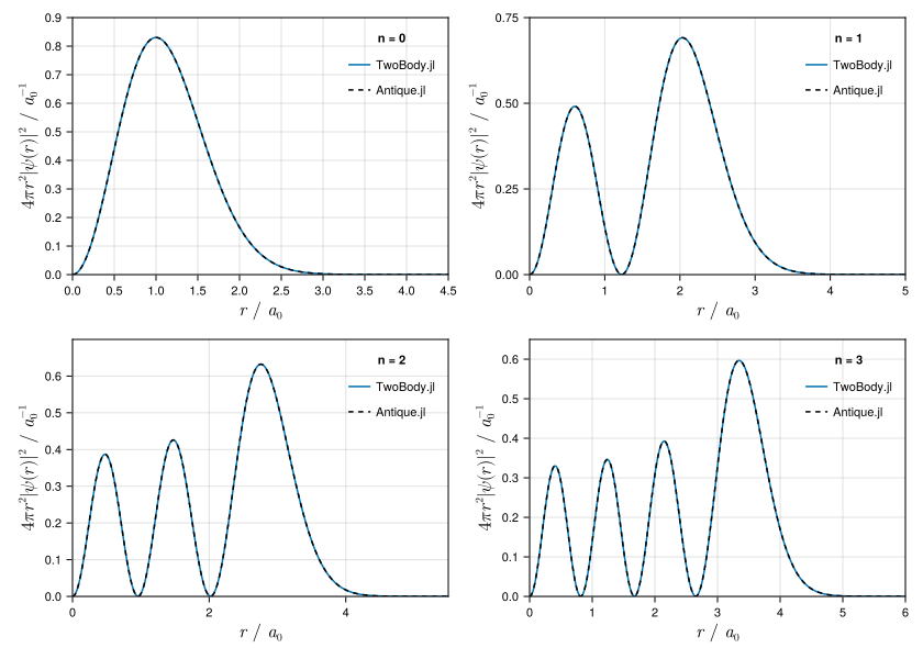
STO-3G
This example reproduces the STO-3G calculation for hydrogen reported by Pérez-Torres (2019). In the contracted calculation, the published coefficients are held fixed, and the resulting contracted function is supplied to the solver. In the uncontracted calculation, the three primitive functions are supplied separately, allowing the Rayleigh–Ritz solver to optimize their linear coefficients.
using TwoBody

# Hamiltonian
H = Hamiltonian(
  Kinetic(hbar=1.0, m=1.0),
  Coulomb(coefficient=-1.0),
)

# parameters
α = (0.109818, 0.405771, 2.227660)
C = (0.444635, 0.535328, 0.154329)

# basis set
primitives = ntuple(i -> SimpleGaussianBasis(α[i]), 3)
normalization = ntuple(i -> (2α[i] / π)^(3/4), 3)
coefficients = ntuple(i -> C[i] * normalization[i], 3)
contracted_basis = ContractedBasis(coefficients, primitives)

# solve
contracted = solve(H, BasisSet(contracted_basis))
uncontracted = solve(H, BasisSet(primitives...))

# results
println("Contracted STO-3G")
println("  This work: ", contracted.E[1])
println("  Reference: ", -0.494908)
println("Uncontracted STO-3G")
println("  This work: ", uncontracted.E[1])
println("  Reference: ", -0.495010)
Contracted STO-3G
This work: -0.49490709657047555
Reference: -0.494908
Uncontracted STO-3G
This work: -0.49501040201217517
Reference: -0.49501The results agree with those in Table 1 of the Supporting Information. The small differences between the calculated and reference values arise from rounding in the published parameters.
Custom Potential
The Hamiltonian can be flexibly customized for applications in quark models. If the potential you need is not implemented in Hamiltonian.jl, you can define it yourself using Custom. However, since this involves numerical integration, both speed and accuracy will be reduced.
using Printf
using TwoBody

H_coulomb = Hamiltonian(
  Kinetic(hbar = 1, m = 1),
  Coulomb(coefficient = -1),
)

H_custom = Hamiltonian(
  Kinetic(hbar = 1, m = 1),
  Custom(r -> -1/r),
)

BS = BasisSet(
  SimpleGaussianBasis(13.00773),
  SimpleGaussianBasis(1.962079),
  SimpleGaussianBasis(0.444529),
  SimpleGaussianBasis(0.1219492),
)

resutl_coulomb = solve(H_coulomb, BS)
resutl_custom = solve(H_custom, BS)

println(" n       Coulomb        Custom")
println("--  ------------  ------------")
for i in 1:4
  @printf("%2d  %+.9f  %+.9f\n", i, resutl_coulomb.E[i], resutl_custom.E[i])
end
n Coulomb Custom
-- ------------ ------------
1 -0.499278406 -0.499278406
2 +0.113213920 +0.113213920
3 +2.592299572 +2.592299572
4 +21.144365190 +21.144365190API reference
Solver
TwoBody.solve — Method
solve(hamiltonian::Hamiltonian, basisset::BasisSet)
This function returns the eigenvalues $E$ and eigenvectors $\pmb{c}$ for
\[\pmb{H} \pmb{c} = E \pmb{S} \pmb{c}.\]
The Hamiltonian matrix is defined as $H_{ij} = \langle \phi_{i} | \hat{H} | \phi_{j} \rangle$. The overlap matrix is defined as $S_{ij} = \langle \phi_{i} | \phi_{j} \rangle$.
TwoBody.solve — Method
solve(hamiltonian::Hamiltonian, basis::Basis; perturbation=Hamiltonian(), info=4)
This a solver for 1-basis calculations. This function returns solve(hamiltonian, BasisSet(basis); perturbation=perturbation, info=info).
TwoBody.solve — Method
solve(hamiltonian::Hamiltonian, basisset::GeometricBasisSet; perturbation=Hamiltonian(), info=4)
This function is a wrapper for solve(hamiltonian::Hamiltonian, basisset::BasisSet, ...).
TwoBody.optimize — Method
function optimize(hamiltonian::Hamiltonian, basisset::BasisSet; perturbation=Hamiltonian(), info=4, progress=true, optimizer=Optim.NelderMead(), options...)
This function minimizes the energy by changing the exponents of the basis functions using Optim.jl.
\[\frac{\partial E}{\partial a_i} = 0\]
TwoBody.optimize — Method
optimize(hamiltonian::Hamiltonian, basis::Basis; perturbation=Hamiltonian(), info=4, optimizer=Optim.NelderMead())
This a optimizer for 1-basis calculations. This function returns optimize(hamiltonian, BasisSet(basis); perturbation=perturbation, info=info, progress=progress, optimizer=optimizer, options...).
TwoBody.optimize — Method
optimize(hamiltonian::Hamiltonian, basisset::GeometricBasisSet; perturbation=Hamiltonian(), info=4, optimizer=Optim.NelderMead())
This function minimizes the energy by optimizing $r_1$ and $r_n$ using Optim.jl.
\[\frac{\partial E}{\partial r_1} = \frac{\partial E}{\partial r_n} = 0\]
Basis Set
TwoBody.BasisSet — Type
BasisSet(basis1, basis2, ...)
\[\{ \phi_1, \phi_2, \phi_3, \cdots \}\]
The basis set is the input for Rayleigh-Ritz method. You can define the basis set like this:
The concrete element type is preserved when all basis functions have a common type, avoiding abstract Basis dispatch in matrix-construction loops.
\[\begin{aligned} \phi_1(r) &= \exp(-13.00773 ~r^2), \\ \phi_2(r) &= \exp(-1.962079 ~r^2), \\ \phi_3(r) &= \exp(-0.444529 ~r^2), \\ \phi_4(r) &= \exp(-0.1219492 ~r^2). \end{aligned}\]
BS = BasisSet(
  SimpleGaussianBasis(13.00773),
  SimpleGaussianBasis(1.962079),
  SimpleGaussianBasis(0.444529),
  SimpleGaussianBasis(0.1219492),
)TwoBody.GeometricBasisSet — Type
GeometricBasisSet(basistype, r₁, rₙ, n; nₘᵢₙ=1, nₘₐₓ=n)
This is a basis set with exponents generated by geometric(r₁, rₙ, n; nₘₐₓ=n, nₘᵢₙ=1). You can define the 20 real-range Gaussian basis functions used for the hydrogen atom in Appendix A.2 and Table VII of E. Hiyama, M. Kamimura, Front. Phys. 13, 132106 (2018) like this:
\[ r_1 = 0.1, r_{n_\mathrm{max}} = 80.0, n_\mathrm{max} = 20.\]
BS = GeometricBasisSet(GaussianBasis, 0.1, 80.0, 20)TwoBody.geometric — Method
geometric(r₁, rₙ, n::Int; nₘₐₓ::Int=n, nₘᵢₙ::Int=1)
Exponents of Gaussian basis functions are given by geometric progression:
\[\begin{aligned} & v_i = \frac{1}{r_i^2}, \\ & r_i = r_1 a^{i-1}. \end{aligned}\]
This function return array of $\nu_i$:
\[(r_1, r_{n}, n, n_\mathrm{max}) \mapsto (\nu_1, \nu_2, \cdots, \nu_{n-1}, \nu_n, \nu_{n+1}, \cdots, \nu_{n_\mathrm{max}})\]
Usually $n = n_\mathrm{max}$. Set $n<n_\mathrm{max}$ if you want to extend the geometric progression.
Examples:
julia> ν = TwoBody.geometric(0.1, 10.0, 5)
5-element Vector{Float64}:
 100.0
  10.0
   0.9999999999999997
   0.09999999999999996
   0.009999999999999995

julia> ν = TwoBody.geometric(0.1, 10.0, 5, nₘₐₓ = 10)
10-element Vector{Float64}:
 100.0
  10.0
   0.9999999999999997
   0.09999999999999996
   0.009999999999999995
   0.0009999999999999994
   9.999999999999994e-5
   9.999999999999992e-6
   9.999999999999991e-7
9.999999999999988e-8Basis Functions
TwoBody.SimpleGaussianBasis — Type
SimpleGaussianBasis(a=1)
Position-Space
\[\phi_i(\pmb{r}) = \exp(-a_i r^2)\]
Momentum-Space
\[\phi_{i}(\pmb{k}) = \frac{1}{(2a_i)^{\frac{3}{2}}} \exp(-k^2/4a_i)\]
Proof (Fourier Transform)
\[\begin{aligned} \phi_{n}(\pmb{k}) &= \frac{1}{\sqrt{2 \pi}^3} \int \phi_{n}(\pmb{r}) \mathrm{e}^{\mathrm{i} \pmb{k} \cdot \pmb{r}} \mathrm{d}\pmb{r} \\ &= \frac{1}{\sqrt{2 \pi}^3} \int \phi_{n}(\pmb{r}) \mathrm{e}^{\mathrm{i} \pmb{k} \cdot \pmb{r}} r^2 \sin (\theta) ~\mathrm{d}r \mathrm{d}\theta \mathrm{d} \varphi \\ &= \frac{1}{\sqrt{2 \pi}^3} \iiint \mathrm{e}^{-\alpha_i r^2} \sqrt{4\pi} Y_{00}(\hat{\pmb{r}}) \left[ 4 \pi \sum_{l'=0}^{\infty} \sum_{m=-l'}^{l'} \mathrm{i}^{l'} j_{l'}(pr) Y_{l'm'}(\hat{\pmb{k}}) Y_{l'm'}^*(\hat{\pmb{r}}) \right] r^2 \sin\theta~ \mathrm{d} r \mathrm{d} \theta \mathrm{d} \varphi \\ &= \frac{1}{\sqrt{2 \pi}^3} 4 \pi \sqrt{4\pi} \sum_{l'=0}^{\infty} \sum_{m=-l'}^{l'} \left[ \mathrm{i}^{l'} Y_{l'm'}(\hat{\pmb{k}}) \int_0^{2 \pi} \int_0^\pi Y_{00}(\hat{\pmb{r}}) Y_{l'm'}^*(\hat{\pmb{r}}) \sin (\theta)~ \mathrm{d} \theta \mathrm{d} \varphi \int_0^{\infty} j_{l'}(pr) \mathrm{e}^{-\alpha_i r^2} r^{2} \mathrm{d}r \right]\\ &= \frac{1}{\sqrt{2 \pi}^3} 4 \pi \sqrt{4\pi} \sum_{l'=0}^{\infty} \sum_{m=-l'}^{l'} \left[ \mathrm{i}^{l'} Y_{l'm'}(\hat{\pmb{k}}) \delta_{0l'} \delta_{0m'} \int_0^{\infty} j_{l'}(kr) \mathrm{e}^{-\alpha_i r^2} r^{2} \mathrm{d}r \right] \\ &= \frac{1}{\sqrt{2 \pi}^3} 4 \pi \sqrt{4\pi} \mathrm{i}^{0} Y_{00}(\hat{\pmb{k}}) \int_0^{\infty} j_{0}(kr) \mathrm{e}^{-\alpha_i r^2} r^{2} \mathrm{d}r \\ &= \frac{1}{2\pi\sqrt{2\pi}} 4 \pi \frac{\sqrt{4\pi}}{\sqrt{4\pi}} \sqrt{\frac{\pi}{2}} \sqrt{\frac{2}{\pi}} \int_0^{\infty} j_{0}(kr) \mathrm{e}^{-\alpha_i r^2} r^{2} ~\mathrm{d}r \\ &= \frac{1}{(2\alpha_i)^{\frac{3}{2}}} \mathrm{e}^{-\frac{k^2}{4 \alpha_i}} \end{aligned}\]
Formula
plane-wave expansion in spherical harmonics:
\[\mathrm{e}^{\mathrm{i} \pmb{k} \cdot \pmb{r}} = 4 \pi \sum_{l=0}^{\infty} \sum_{m=-l}^{l} \mathrm{i}^{l} j_{l}(pr) Y_{lm}(\hat{\pmb{k}}) Y_{lm}^*(\hat{\pmb{r}})\]
special case of spherical harmonics:
\[Y_{00}(\hat{\pmb{r}}) = \frac{1}{\sqrt{4\pi}}\]
orthonormality of spherical harmonics:
\[\int_0^{2\pi} \int_0^\pi Y_{lm}(\hat{\pmb{r}})^* Y_{l'm'}(\hat{\pmb{r}}) \sin(\theta) ~ \mathrm{d} \theta \mathrm{d} \varphi = \delta_{ll'} \delta_{mm'}\]
citation needed:
\[\sqrt{\frac{2}{\pi}} \int r^{l} j_l(kr) \mathrm{e}^{-\alpha r^2} r^{2} \mathrm{d} r = \frac{1}{(2\alpha)^{l+\frac{3}{2}}} k^l e^{-\frac{k^2}{4\alpha}}\]
TwoBody.ContractedBasis — Type
ContractedBasis([c1, c2, ...], [primitive1, primitive2, ...])
\[\phi' = \sum_i c_i \phi_i\]
A contracted basis is a nonempty linear combination of PrimitiveBasis objects. The numbers of coefficients and primitive bases must match. Numeric coefficient types are promoted to a common type.
The components are stored in tuples, making their number part of the type and preserving the concrete type of every primitive basis. This lets Julia specialize and inline evaluation without dispatching through an abstract PrimitiveBasis container. Tuple inputs are recommended when constructing a basis in performance-sensitive code; vectors are also accepted and converted once during construction.
The fields are named coefficients and primitives. The aliases c and φ are retained for compatibility.
Matrix
TwoBody.matrix — Method
matrix(basisset::BasisSet)
This function returns the overlap matrix $\pmb{S}$. The element is written as $S_{ij} = \langle \phi_{i} | \phi_{j} \rangle$.
TwoBody.matrix — Method
matrix(operator::Operator, basisset::BasisSet)
This function is used for the expectation values and is not used in computing the Hamiltonian matrix.
This function returns the matrix corresponding to the operator in the given basis set. The element is written as $O_{ij} = \langle \phi_{i} | \hat{o} | \phi_{j} \rangle$.
TwoBody.matrix — Method
matrix(hamiltonian::Hamiltonian, basisset::BasisSet)
This function returns the Hamiltonian matrix $\pmb{H}$. The element is written as $H_{ij} = \langle \phi_{i} | \hat{H} | \phi_{j} \rangle$.
Matrix Elements
TwoBody.element — Method
element(SGB1::SimpleGaussianBasis, SGB2::SimpleGaussianBasis)
\[\begin{aligned} S_{ij} = \langle \phi_{i} | \phi_{j} \rangle &= \int \phi_{i}^*(r) \phi_{j}(r) \mathrm{d} \pmb{r} \\ &= \iiint \mathrm{e}^{-\alpha_i r^2} \mathrm{e}^{-\alpha_j r^2} ~r^2 \sin\theta ~ \mathrm{d} r \mathrm{d} \theta \mathrm{d} \varphi \\ &= \int_0^{2\pi} \mathrm{d}\varphi \int_0^\pi \sin\theta ~\mathrm{d}\theta \int_0^\infty r^{2} \mathrm{e}^{-(\alpha_i + \alpha_j) r^2} ~\mathrm{d}r \\ &= 2\pi \times 2 \times \frac{1!!}{2^{2}} \sqrt{\frac{\pi}{a^{3}}} \\ &= \underline{\left( \frac{\pi}{\alpha_i + \alpha_j} \right)^{3/2}} \end{aligned}\]
Integral Formula:
\[\int_0^{\infty} r^{2n} \exp \left(-a r^2\right) ~\mathrm{d}r = \frac{(2n-1)!!}{2^{n+1}} \sqrt{\frac{\pi}{a^{2n+1}}}\]
TwoBody.element — Method
element(o::Hamiltonian, SGB1::SimpleGaussianBasis, SGB2::SimpleGaussianBasis)
\[\begin{aligned} H_{ij} &= \langle \phi_{i} | \hat{H} | \phi_{j} \rangle \\ &= \langle \phi_{i} | \sum_k \hat{o}_k | \phi_{j} \rangle \\ &= \sum_k \langle \phi_{i} | \hat{o}_k | \phi_{j} \rangle \\ \end{aligned}\]
TwoBody.element — Method
element(o::RestEnergy, SGB1::SimpleGaussianBasis, SGB2::SimpleGaussianBasis)
\[\begin{aligned} \langle \phi_{i} | mc^2 | \phi_{j} \rangle &= mc^2 \langle \phi_{i} | \phi_{j} \rangle \\ &= mc^2 \iiint \phi_{i}^*(r) \phi_{j}(r) ~r^2 \sin\theta ~\mathrm{d}r \mathrm{d}\theta \mathrm{d}\varphi \\ &= mc^2 \int_0^{2\pi} \mathrm{d}\varphi \int_0^\pi \sin\theta ~\mathrm{d}\theta \int_0^\infty r^{2} \mathrm{e}^{-(\alpha_i + \alpha_j) r^2} ~\mathrm{d}r \\ &= mc^2 \times 2\pi \times 2 \times \frac{1!!}{2^{2}} \sqrt{\frac{\pi}{a^{3}}} \\ &= \underline{mc^2 \left( \frac{\pi}{\alpha_i + \alpha_j} \right)^{3/2}} \end{aligned}\]
Integral Formula:
\[\int_0^{\infty} r^{2n} \exp \left(-a r^2\right) ~\mathrm{d}r = \frac{(2n-1)!!}{2^{n+1}} \sqrt{\frac{\pi}{a^{2n+1}}}\]
TwoBody.element — Method
element(o::Laplacian, SGB1::SimpleGaussianBasis, SGB2::SimpleGaussianBasis)
\[\begin{aligned} \langle \phi_{i} | \nabla^2 | \phi_{j} \rangle = \underline{ -6 \frac{\alpha_i \alpha_j \pi^{\frac{3}{2}}}{(\alpha_i + \alpha_j)^{\frac{5}{2}}} } \end{aligned}\]
TwoBody.element — Method
element(o::Kinetic, SGB1::SimpleGaussianBasis, SGB2::SimpleGaussianBasis)
Derivation (without Green's identity)
\[\begin{aligned} T_{ij} = \langle \phi_{i} | \hat{T} | \phi_{j} \rangle &= \iiint \mathrm{e}^{-\alpha_i r^2} \left[ -\frac{\hbar^2}{2\mu} \nabla^2 \right] \mathrm{e}^{-\alpha_j r^2} ~r^2 \sin\theta ~\mathrm{d}r \mathrm{d}\theta \mathrm{d}\varphi \\ &= -\frac{\hbar^2}{2\mu} \iiint \mathrm{e}^{-\alpha_i r^2} \left[ \nabla^2 \right] \mathrm{e}^{-\alpha_j r^2} ~r^2 \sin\theta ~\mathrm{d}r \mathrm{d}\theta \mathrm{d}\varphi \\ &= -\frac{\hbar^2}{2\mu} \iiint \mathrm{e}^{-\alpha_i r^2} \left[ -6\alpha_j + 4\alpha_j^2 r^2 \right] \mathrm{e}^{-\alpha_j r^2} ~r^2 \sin\theta ~\mathrm{d}r \mathrm{d}\theta \mathrm{d}\varphi \\ &= -\frac{\hbar^2}{2\mu} \iint \sin\theta ~\mathrm{d}\theta \mathrm{d}\varphi \int \left[ -6\alpha_j + 4\alpha_j^2 r^2 \right] r^2 \mathrm{e}^{-(\alpha_i + \alpha_j) r^2} ~\mathrm{d}r \\ &= -\frac{\hbar^2}{2\mu} \cdot 4\pi \left[ -6\alpha_j \mathrm{GGI}(2, \alpha_i + \alpha_j) +4\alpha_j^2 \mathrm{GGI}(4, \alpha_i + \alpha_j) \right] \\ &= -\frac{\hbar^2}{2\mu} \cdot 4\pi \left[ -6\alpha_j \frac{\Gamma\left( \frac{3}{2} \right)}{2 (\alpha_i + \alpha_j)^{\frac{3}{2}}} +4\alpha_j^2 \frac{\Gamma\left( \frac{5}{2} \right)}{2 (\alpha_i + \alpha_j)^{\frac{5}{2}}} \right] \\ &= -\frac{\hbar^2}{2\mu} \cdot 4\pi \left[ -6\alpha_j \frac{ \sqrt{\pi}/2}{2 (\alpha_i + \alpha_j)^{\frac{3}{2}}} +4\alpha_j^2 \frac{3\sqrt{\pi}/4}{2 (\alpha_i + \alpha_j)^{\frac{5}{2}}} \right] \\ &= -\frac{\hbar^2}{2\mu} \cdot 4\pi \left[ \frac{\alpha_j}{\alpha_i + \alpha_j} - 1 \right] \cdot 6 \alpha_j \cdot \frac{\sqrt{\pi}/2}{2 (\alpha_i + \alpha_j)^{\frac{3}{2}}} \\ &= -\frac{\hbar^2}{2\mu} \cdot 4\pi \left[ - \frac{\alpha_i}{\alpha_i + \alpha_j} \right] \cdot 6 \alpha_j \cdot \frac{\sqrt{\pi}/2}{2 (\alpha_i + \alpha_j)^{\frac{3}{2}}} \\ &= \underline{ \frac{\hbar^2}{2\mu} \cdot 6 \cdot \frac{\alpha_i \alpha_j \pi^{\frac{3}{2}}}{(\alpha_i + \alpha_j)^{\frac{5}{2}}} } \end{aligned}\]
Derivation (with Green's identity)
\[\begin{aligned} T_{ij} = \langle \phi_{i} | \hat{T} | \phi_{j} \rangle &= \iiint \mathrm{e}^{-\alpha_i r^2} \left[ -\frac{\hbar^2}{2\mu} \nabla^2 \right] \mathrm{e}^{-\alpha_j r^2} ~r^2 \sin\theta ~\mathrm{d}r \mathrm{d}\theta \mathrm{d}\varphi \\ &= -\frac{\hbar^2}{2\mu} \iiint \mathrm{e}^{-\alpha_i r^2} \nabla^2 \mathrm{e}^{-\alpha_j r^2} ~r^2 \sin\theta ~\mathrm{d}r \mathrm{d}\theta \mathrm{d}\varphi \\ &= \frac{\hbar^2}{2\mu} \iiint \left[ \nabla \mathrm{e}^{-\alpha_i r^2} \right] \left[ \nabla \mathrm{e}^{-\alpha_j r^2} \right] ~r^2 \sin\theta ~\mathrm{d}r \mathrm{d}\theta \mathrm{d}\varphi \\ &= \frac{\hbar^2}{2\mu} \iiint \left[ -2 \alpha_i r \mathrm{e}^{-\alpha_i r^2} \right] \left[ -2 \alpha_j r \mathrm{e}^{-\alpha_j r^2} \right] ~r^2 \sin\theta ~\mathrm{d}r \mathrm{d}\theta \mathrm{d}\varphi \\ &= \frac{\hbar^2}{2\mu} \cdot 4 \alpha_i \alpha_j \iiint \left[ r \mathrm{e}^{-\alpha_i r^2} \right] \left[ r \mathrm{e}^{-\alpha_j r^2} \right] ~r^2 \sin\theta ~\mathrm{d}r \mathrm{d}\theta \mathrm{d}\varphi \\ &= \frac{\hbar^2}{2\mu} \cdot 4 \alpha_i \alpha_j \iint \sin\theta ~\mathrm{d}\theta \mathrm{d}\varphi \int r^4 \mathrm{e}^{- (\alpha_i + \alpha_j) r^2} ~\mathrm{d}r \\ &= \frac{\hbar^2}{2\mu} \cdot 4 \alpha_i \alpha_j \cdot 4 \pi \cdot \mathrm{GGI}(4, \alpha_i + \alpha_j) \\ &= \frac{\hbar^2}{2\mu} \cdot 4 \alpha_i \alpha_j \cdot 4 \pi \cdot \frac{\Gamma\left( \frac{5}{2} \right)}{2 (\alpha_i + \alpha_j)^{\frac{5}{2}}} \\ &= \frac{\hbar^2}{2\mu} \cdot 4 \alpha_i \alpha_j \cdot 4 \pi \cdot \frac{3\sqrt{\pi}/4}{2 (\alpha_i + \alpha_j)^{\frac{5}{2}}} \\ &= \underline{ \frac{\hbar^2}{2\mu} \cdot 6 \cdot \frac{\alpha_i \alpha_j \pi^{\frac{3}{2}}}{(\alpha_i + \alpha_j)^{\frac{5}{2}}} } \end{aligned}\]
Formula
\[\begin{aligned} \iiint_V f \pmb{\nabla}^2 g ~ \mathrm{d}V + \iiint_V \pmb{\nabla} f \cdot \pmb{\nabla} g ~ \mathrm{d}V = \iint_{\partial V} f \pmb{\nabla} g \cdot \pmb{n} ~ \mathrm{d}S \end{aligned}\]
generalized Gaussian integral:
\[\begin{aligned} \mathrm{GGI}(n,b) = \int_0^{\infty} x^{n} \exp \left(-b x^2\right) \mathrm{d}x = \frac{\Gamma\left( \frac{n+1}{2} \right)}{2 b^{\frac{n+1}{2}}} \end{aligned}\]
TwoBody.element — Method
element(o::Constant, SGB1::SimpleGaussianBasis, SGB2::SimpleGaussianBasis)
\[\begin{aligned} \langle \phi_{i} | c | \phi_{j} \rangle &= c \langle \phi_{i} | \phi_{j} \rangle \\ &= c \iiint \phi_{i}^*(r) \phi_{j}(r) ~r^2 \sin\theta ~\mathrm{d}r \mathrm{d}\theta \mathrm{d}\varphi \\ &= c \int_0^{2\pi} \mathrm{d}\varphi \int_0^\pi \sin\theta ~\mathrm{d}\theta \int_0^\infty r^{2} \mathrm{e}^{-(\alpha_i + \alpha_j) r^2} ~\mathrm{d}r \\ &= c \times 2\pi \times 2 \times \frac{1!!}{2^{2}} \sqrt{\frac{\pi}{a^{3}}} \\ &= \underline{c \left( \frac{\pi}{\alpha_i + \alpha_j} \right)^{3/2}} \end{aligned}\]
Integral Formula:
\[\int_0^{\infty} r^{2n} \exp \left(-a r^2\right) ~\mathrm{d}r = \frac{(2n-1)!!}{2^{n+1}} \sqrt{\frac{\pi}{a^{2n+1}}}\]
TwoBody.element — Method
element(o::Linear, SGB1::SimpleGaussianBasis, SGB2::SimpleGaussianBasis)
\[\begin{aligned} \langle \phi_{i} | r | \phi_{j} \rangle &= \iiint \phi_{i}^*(r) \times r \times \phi_{j}(r) ~r^2 \sin\theta ~\mathrm{d}r \mathrm{d}\theta \mathrm{d}\varphi \\ &= \int_0^{2\pi} \mathrm{d}\varphi \int_0^\pi \sin\theta ~\mathrm{d}\theta \int_0^\infty r^3 \mathrm{e}^{-(\alpha_i + \alpha_j) r^2} ~\mathrm{d}r \\ &= 2\pi \times 2 \times \frac{1!}{2 (\alpha_i + \alpha_j)^{2}} \\ &= \underline{\frac{2\pi}{(\alpha_i + \alpha_j)^2}} \end{aligned}\]
Integral Formula:
\[\int_0^{\infty} r^{2n+1} \exp \left(-a r^2\right) ~\mathrm{d}r = \frac{n!}{2 a^{n+1}}\]
TwoBody.element — Method
element(o::Coulomb, SGB1::SimpleGaussianBasis, SGB2::SimpleGaussianBasis)
\[\begin{aligned} \langle \phi_{i} | \frac{1}{r} | \phi_{j} \rangle &= \iiint \phi_{i}^*(r) \times \frac{1}{r} \times \phi_{j}(r) ~r^2 \sin\theta ~\mathrm{d}r \mathrm{d}\theta \mathrm{d}\varphi \\ &= \int_0^{2\pi} \mathrm{d}\varphi \int_0^\pi \sin\theta ~\mathrm{d}\theta \int_0^\infty r \mathrm{e}^{-(\alpha_i + \alpha_j) r^2} ~\mathrm{d}r \\ &= 2\pi \times 2 \times \frac{0!}{2 (\alpha_i + \alpha_j)} \\ &= \underline{\frac{2\pi}{\alpha_i + \alpha_j}} \end{aligned}\]
Integral Formula:
\[\int_0^{\infty} r^{2n+1} \exp \left(-a r^2\right) ~\mathrm{d}r = \frac{n!}{2 a^{n+1}}\]
TwoBody.element — Method
element(o::PowerLaw, SGB1::SimpleGaussianBasis, SGB2::SimpleGaussianBasis)
\[\begin{aligned} \langle \phi_{i} | r^n | \phi_{j} \rangle &= \iiint \phi_{i}^*(r) \times r^n \times \phi_{j}(r) ~r^2 \sin\theta ~\mathrm{d}r \mathrm{d}\theta \mathrm{d}\varphi \\ &= \int_0^{2\pi} \mathrm{d}\varphi \int_0^\pi \sin\theta ~\mathrm{d}\theta \int_0^\infty r^{n+2} \mathrm{e}^{-(\alpha_i + \alpha_j) r^2} ~\mathrm{d}r \\ &= 2\pi \times 2 \times \frac{\Gamma\left( \frac{n+3}{2} \right)}{2 (\alpha_i + \alpha_j)^{\frac{n+3}{2}}} \\ &= \underline{2\pi\frac{\Gamma\left( \frac{n+3}{2} \right)}{(\alpha_i + \alpha_j)^{\frac{n+3}{2}}}} \end{aligned}\]
Integral Formula:
\[\int_0^{\infty} r^{n} \exp \left(-a r^2\right) ~\mathrm{d}r = \frac{\Gamma\left( \frac{n+1}{2} \right)}{2 a^{\frac{n+1}{2}}}\]
TwoBody.element — Method
element(o::Gaussian, SGB1::SimpleGaussianBasis, SGB2::SimpleGaussianBasis)
\[\begin{aligned} \langle \phi_{i} | \exp(-br^2) | \phi_{j} \rangle &= \iiint \phi_{i}^*(r) \times \exp(-br^2) \times \phi_{j}(r) ~r^2 \sin\theta ~\mathrm{d}r \mathrm{d}\theta \mathrm{d}\varphi \\ &= \int_0^{2\pi} \mathrm{d}\varphi \int_0^\pi \sin\theta ~\mathrm{d}\theta \int_0^\infty r^2 \mathrm{e}^{-(b+\alpha_i + \alpha_j) r^2} ~\mathrm{d}r \\ &= 2\pi \times 2 \times \frac{1!!}{2^{2}} \sqrt{\frac{\pi}{(b + \alpha_i + \alpha_j)^{2\cdot1+1}}} \\ &= \underline{\left( \frac{\pi}{b + \alpha_i + \alpha_j} \right)^{3/2}} \end{aligned}\]
Integral Formula:
\[\int_0^{\infty} r^{2n} \exp \left(-a r^2\right) ~\mathrm{d}r = \frac{(2n-1)!!}{2^{n+1}} \sqrt{\frac{\pi}{a^{2n+1}}}\]
TwoBody.element — Method
element(o::Custom, SGB1::SimpleGaussianBasis, SGB2::SimpleGaussianBasis)
The matrix element for a custom central potential is evaluated numerically with adaptive Gauss–Kronrod quadrature:
\[\langle \phi_i | V | \phi_j \rangle = 4\pi \int_0^\infty r^2 \phi_i(r) V(r) \phi_j(r)\,\mathrm{d}r.\]