Finite Difference Method

This method solve the eigenvalue problem for the Hamiltonian discretized as a sparse matrix with finite difference approximation,

\[\pmb{H} \pmb{\psi} = E \pmb{\psi}.\]

The eigenvalue $E$ is an approximation of the exact energy and the eigenvector $\pmb{\psi}$ is a vector of the approximated values of the exact wavefunction $\psi(r)$ on points of the grid,

\[\pmb{\psi} = \left(\begin{array}{c} \psi(r_1) \\ \psi(r_2) \\ \psi(r_3) \\ \vdots \\ \end{array}\right).\]

A uniform grid spacing is used, $r_{i+1} = r_{i} + \Delta r$. See the API reference for the expression of the matrix $\pmb{H}$.

Usage

Run the following code before each use.

using TwoBody

Define the Hamiltoninan. This is an example for the non-relativistic Hamiltonian of hydrogen atom in atomic units:

\[\hat{H} = - \frac{1}{2} \nabla^2 - \frac{1}{r}\]

H = Hamiltonian(
  Kinetic(hbar = 1, m = 1),
  Coulomb(coefficient = -1),
)

Set the calculation options.

FDM = FiniteDifferenceMethod(
  Δr = 0.1,
  rₘₐₓ = 50.0,
  l = 0,
  direction = :c,
  solver = :LinearAlgebra,
)

Solve the eigenvalue problem. You should find reasonable approximations to the exact eigenvalues:

\[\begin{aligned} E_{n=1} &= -0.5,\\ E_{n=2} &= -0.125,\\ E_{n=3} &= -0.05555\cdots,\\ E_{n=4} &= -0.03125. \end{aligned}\]

By default the eigenvalues and the expectation values are displayed.

julia> solve(H, FDM)
# method

FiniteDifferenceMethod(Δr=0.1, rₘₐₓ=50.0, R=0.1:0.1:50.0, l=0, direction=c, solver=LinearAlgebra)

# eigenvalue

E₁ = -0.4987562112092615
E₂ = -0.12492197250369766
E₃ = -0.05554012469051319
E₄ = -0.031200723331266493

# others

n 	norm, <ψₙ|ψₙ> = cₙ' * cₙ
1	0.9999999999999998
2	0.9999999999999999
3	1.0000000000000004
4	1.0

n 	error check, |<ψₙ|H|ψₙ> - E| = |cₙ' * H * cₙ - E| = 0
1	3.673727988484643e-13
2	2.2917778785824794e-13
3	2.5460883401606793e-13
4	2.530718690163525e-13

n 	expectation value of Kinetic(hbar=1, m=1)
1	3.2786923701708206
2	3.530703114153333
3	3.5759997979300326
4	3.5934083915850286

n 	expectation value of Coulomb(coefficient=-1)
1	-3.777448581379713
2	-3.655625086656795
3	-3.631539922620289
4	-3.6246091149160358

(hamiltonian = Hamiltonian(Kinetic(hbar=1, m=1), Coulomb(coefficient=-1)), perturbation = Hamiltonian(), method = FiniteDifferenceMethod(Δr=0.1, rₘₐₓ=50.0, R=0.1:0.1:50.0, l=0, direction=c, solver=LinearAlgebra), nₘₐₓ = 4, H = sparse([1, 2, 1, 2, 3, 2, 3, 4, 3, 4  …  497, 498, 497, 498, 499, 498, 499, 500, 499, 500], [1, 1, 2, 2, 2, 3, 3, 3, 4, 4  …  497, 497, 498, 498, 498, 499, 499, 499, 500, 500], [89.99999999999999, -24.999999999999993, -100.0, 94.99999999999999, -33.33333333333333, -75.0, 96.66666666666666, -37.49999999999999, -66.66666666666666, 97.49999999999999  …  99.97987927565391, -49.89959839357429, -50.10060362173037, 99.97991967871485, -49.89979959919839, -50.1004016064257, 99.97995991983967, -49.89999999999999, -50.1002004008016, 99.97999999999999], 500, 500), J = sparse([1, 2, 3, 4, 5, 6, 7, 8, 9, 10  …  491, 492, 493, 494, 495, 496, 497, 498, 499, 500], [1, 2, 3, 4, 5, 6, 7, 8, 9, 10  …  491, 492, 493, 494, 495, 496, 497, 498, 499, 500], [0.010000000000000002, 0.04000000000000001, 0.09, 0.16000000000000003, 0.25, 0.36, 0.48999999999999994, 0.6400000000000001, 0.81, 1.0  …  2410.81, 2420.6400000000003, 2430.49, 2440.3599999999997, 2450.25, 2460.1600000000003, 2470.09, 2480.0399999999995, 2490.0099999999998, 2500.0], 500, 500), E = [-0.4987562112092615, -0.12492197250369766, -0.05554012469051319, -0.031200723331266493], C = [0.4254380241849766 0.4251461161934448 0.4250919140636053 -0.4251709606200608; 0.3850161203369446 0.38316260548846925 0.3828188192363622 -0.3827865209731601; … ; 1.9041443531396908e-17 -2.778714615755565e-11 4.3280324837293224e-7 3.851240744573792e-5; -1.1836573006003485e-16 -1.3851685999590626e-11 2.158920922815757e-7 1.9215539036411178e-5], ψ = [0.5093160129260603 0.1803838291995552 0.09822040734929309 -0.06432384275343007; 0.460924656882603 0.1625707853171123 0.08845291835107645 -0.05791152798230022; … ; 2.2795593126276707e-17 -1.178971566600631e-11 1.000021641223832e-7 5.826517495416151e-6; -1.417023356498282e-16 -5.877085703728113e-12 4.988335121381465e-8 2.9071066132972178e-6])

Example of Hydrogen Atom

Analytical solutions are implemented in Antique.jl.

# solve
using TwoBody
H = Hamiltonian(Kinetic(1, 1), Coulomb(-1))
FDM = FiniteDifferenceMethod()
res = solve(H, FDM, info=0, nₘₐₓ=4)

# benchmark
import Antique
HA = Antique.HydrogenAtom(Z=1, E_h=1.0, a_0=1.0, m_e=1.0, hbar=1.0)

# energy
using Printf
println("Total Energy Eₙ")
println("------------------------------")
println(" n     numerical    analytical")
println("------------------------------")
for n in 1:4
  @printf("%2d  %+.9f  %+.9f\n", n, res.E[n], Antique.energy(HA,n=n))
end

# wave function
using CairoMakie
fig = Figure(
  size = (840,600),
  fontsize = 11,
  backgroundcolor = :transparent
)
for n in 1:4
  axis = Axis(
    fig[div(n-1,2)+1,rem(n-1,2)+1],
    xlabel = L"$r~/~a_0$",
    ylabel = L"$4\pi r^2|\psi(r)|^2~ /~{a_0}^{-1}$",
    xlabelsize = 16.5,
    ylabelsize = 16.5,
    limits=(
      0, [5, 15, 30, 50][n],
      0, [0.6, 0.2, 0.11, 0.07][n],
    )
  )
  X = res.method.R
  Y = 4π * X .^2 .* res.ψ[:,n] .^ 2
  scatter!(axis, X, Y, label="TwoBody.jl", markersize=6)
  lines!(axis, 0..50, r -> 4π * r^2 * abs(Antique.wavefunction(HA,r,0,0,n=n))^2, label="Antique.jl", color=:black)
  axislegend(axis, "n = $n", position=:rt, framevisible=false)
end

Total Energy Eₙ
------------------------------
 n     numerical    analytical
------------------------------
 1  -0.498756211  -0.500000000
 2  -0.124921973  -0.125000000
 3  -0.055540125  -0.055555556
 4  -0.031200723  -0.031250000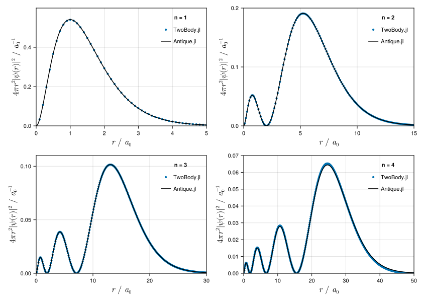

Example of Spherical Oscillator

Analytical solutions are implemented in spherical oscillator.

# solve
using TwoBody
H = Hamiltonian(Kinetic(1, 1), PowerLaw(coefficient=1/2, exponent=2))
FDM = FiniteDifferenceMethod(rₘₐₓ=10.0)
res = solve(H, FDM, info=0, nₘₐₓ=4)

# benchmark
import Antique
SO = Antique.SphericalOscillator(k=1.0, mu=1.0, hbar=1.0)

# energy
using Printf
println("Total Energy Eₙ")
println("------------------------------")
println(" n     numerical    analytical")
println("------------------------------")
for n in 1:4
  @printf("%2d  %+.9f  %+.9f\n", n-1, res.E[n], Antique.energy(SO,n=n-1))
end

# wave function
using CairoMakie
fig = Figure(
  size = (840,600),
  fontsize = 11,
  backgroundcolor = :transparent
)
for n in 1:4
  axis = Axis(
    fig[div(n-1,2)+1,rem(n-1,2)+1],
    xlabel = L"$r~/~a_0$",
    ylabel = L"$4\pi r^2|\psi(r)|^2~ /~{a_0}^{-1}$",
    xlabelsize = 16.5,
    ylabelsize = 16.5,
    limits=(
      0, [4.5, 5.0, 5.5, 6.0][n],
      0, [0.90, 0.75, 0.70, 0.65][n],
    )
  )
  X = res.method.R
  Y = 4π * X .^2 .* res.ψ[:,n] .^ 2
  scatter!(axis, X, Y, label="TwoBody.jl", markersize=6)
  lines!(axis, 0..50, r -> 4π * r^2 * abs(Antique.wavefunction(SO,r,0,0,n=n-1))^2, label="Antique.jl", color=:black)
  axislegend(axis, "n = $(n-1)", position=:rt, framevisible=false)
end
fig

Total Energy Eₙ
------------------------------
 n     numerical    analytical
------------------------------
 0  +1.498435737  +1.500000000
 1  +3.492169621  +3.500000000
 2  +5.480870301  +5.500000000
 3  +7.464518486  +7.500000000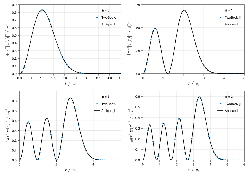

API reference

TwoBody.FiniteDifferenceMethod — Type

FiniteDifferenceMethod(Δr=0.1, rₘₐₓ=50.0, R=Δr:Δr:rₘₐₓ, l=0, direction=:c, solver=:LinearAlgebra)

Arguments	Default	Description
`Δr::Real`	`0.1`	Radial grid spacing. A uniform grid spacing is used, $r_{i+1} = r_{i} + \Delta r$.
`rₘₐₓ::Real`	`50.0`	The maximum value of the radial grid. This value is not directly used in the calculation, but it is used to determine the `R`.
`R::StepRangeLen`	`Δr:Δr:rₘₐₓ`	Radial grid. The origin must be excluded from the grid to avoid divergence of the Coulomb potential and the centrifugal potential at the origin.
`l::Int`	`0`	Angular momentum quantum number. This is a positive integer, $0 \leq l$.
`direction::Symbol`	`:c`	The direction of the finite difference, `:c` for central, :f for forward, `:b` for backward.
`solver::Symbol`	`:LinearAlgebra`	The solver for eigenvalue problem, `:LinearAlgebra` or `:ArnoldiMethod`.

source

TwoBody.solve — Method

solve(hamiltonian::Hamiltonian, method::FiniteDifferenceMethod; perturbation=Hamiltonian(), info=4, nₘₐₓ=4)

This method solve the eigenvalue problem for the Hamiltonian discretized as a sparse matrix with finite difference approximation,

\[\pmb{H} \pmb{\psi} = E \pmb{\psi}.\]

The eigenvalue $E$ is an approximation of the exact energy and the eigenvector $\pmb{\psi}$ is a vector of the approximated values of the exact wavefunction $\psi(r)$ on points of the grid,

\[\pmb{\psi} = \left(\begin{array}{c} \psi(r_1) \\ \psi(r_2) \\ \psi(r_3) \\ \vdots \\ \end{array}\right).\]

source

TwoBody.matrix — Method

matrix(o::Hamiltonian, method::FiniteDifferenceMethod)

The matrix for the Hamiltonian is a sum of matrices for each term,

\[\pmb{H} = \sum_i \pmb{O}_i.\]

source

TwoBody.matrix — Method

matrix(o::RestEnergy, method::FiniteDifferenceMethod)

The matrix for the rest energy $mc^2$ is a diagonal matrix,

\[mc^2 \left(\begin{array}{ccccccc} 1 & 0 & 0 & \ldots \\ 0 & 1 & 0 & \ldots \\ 0 & 0 & 1 & \ldots \\ \vdots & \vdots & \vdots & \ddots \\ \end{array}\right).\]

source

TwoBody.matrix — Method

matrix(o::Kinetic, method::FiniteDifferenceMethod)

We use the shorthand notation $\psi'(r) = \frac{\mathrm{d}\psi}{\mathrm{d}r}(r)$ and $\psi''(r) = \frac{\mathrm{d}^{2}\psi}{\mathrm{d}r^{2}}(r)$. For the uniform grid spacing ($r_{i+1} = r_{i} + \Delta r$), the finite difference for the first derivative,

\[\frac{\mathrm{d}\psi}{\mathrm{d}r}(r) = \frac{\psi(r+\Delta r) - \psi(r-\Delta r)}{2\Delta r} + O(\Delta r^{2})\]

is written as

\[\left(\begin{array}{ccccc} \psi'(r_1) \\ \psi'(r_2) \\ \psi'(r_3) \\ \psi'(r_4) \\ \vdots \end{array}\right) \simeq \frac{1}{2\Delta r} \left(\begin{array}{ccccc} 0 & 1 & 0 & 0 &\ldots \\ -1 & 0 & 1 & 0 &\ldots \\ 0 & -1 & 0 & 1 &\ldots \\ 0 & 0 & -1 & 0 &\ldots \\ \vdots & \vdots & \vdots & \vdots & \ddots \\ \end{array}\right) \left(\begin{array}{ccccccc} \psi(r_1) \\ \psi(r_2) \\ \psi(r_3) \\ \psi(r_4) \\ \vdots \end{array}\right),\]

and the finite difference for the second derivative,

\[\frac{\mathrm{d}^{2}}{\mathrm{d}r^{2}}(r) = \frac{\psi(r+\Delta r) - 2f(r) + \psi(r-\Delta r)}{\Delta r^{2}} + O(\Delta r^{2}).\]

is written as

\[\left(\begin{array}{ccccc} \psi''(r_1) \\ \psi''(r_2) \\ \psi''(r_3) \\ \psi''(r_4) \\ \vdots \end{array}\right) \simeq \frac{1}{\Delta r^2} \left(\begin{array}{ccccccc} -2 & 1 & 0 & 0 & \ldots \\ 1 & -2 & 1 & 0 & \ldots \\ 0 & 1 & -2 & 1 & \ldots \\ 0 & 0 & 1 & -2 & \ldots \\ \vdots & \vdots & \vdots & \vdots & \ddots \end{array}\right) \left(\begin{array}{ccccccc} \psi(r_1) \\ \psi(r_2) \\ \psi(r_3) \\ \psi(r_4) \\ \vdots \end{array}\right).\]

Similarly, the matrix for the kinetic energy,

\[\hat{T} = -\frac{\hbar^2}{2\mu} \left[ \frac{\partial^2}{\partial r^2} + \frac{2}{r} \frac{\partial}{\partial r} - \frac{l(l+1)}{r^2} \right]\]

is written as

\[\pmb{T} = - \frac{\hbar^2}{2\mu} \left[ \frac{1}{{\Delta r}^2} \left(\begin{array}{ccccccc} -2 & 1 & 0 & \ldots \\ 1 & -2 & 1 & \ldots \\ 0 & 1 & -2 & \ldots \\ \vdots & \vdots & \vdots & \ddots \\ \end{array}\right) + \left(\begin{array}{ccccccc} 2/r_1 & 0 & 0 & \ldots \\ 0 & 2/r_2 & 0 & \ldots \\ 0 & 0 & 2/r_3 & \ldots \\ \vdots & \vdots & \vdots & \ddots \\ \end{array}\right) \frac{1}{\Delta r} \left(\begin{array}{ccccccc} 0 & 1 & 0 & \ldots \\ -1 & 0 & 1 & \ldots \\ 0 & -1 & 0 & \ldots \\ \vdots & \vdots & \vdots & \ddots \\ \end{array}\right) - l(l+1) \left(\begin{array}{ccccccc} 1/{r_1}^2 & 0 & 0 & \ldots \\ 0 & 1/{r_2}^2 & 0 & \ldots \\ 0 & 0 & 1/{r_3}^2 & \ldots \\ \vdots & \vdots & \vdots & \ddots \\ \end{array}\right) \right].\]

source

TwoBody.matrix — Method

matrix(o::PotentialTerm, method::FiniteDifferenceMethod)

The matrix for the potential energy $V(r)$ is a diagonal matrix,

\[\pmb{V} = \left(\begin{array}{ccccccc} V(r_1) & 0 & 0 & \ldots \\ 0 & V(r_2) & 0 & \ldots \\ 0 & 0 & V(r_3) & \ldots \\ \vdots & \vdots & \vdots & \ddots \\ \end{array}\right).\]

source