Examples

One-dimensional Metropolis-walk

Note

Even in the one-dimensional case, the initial value must be defined as a vector.

Minimal Working Example for Single-Walker

This is a minimal working example for 1-walker x 1000-steps, 1-dimensional Metropolis-walk on the Gaussian distribution function:

\[p(x) = \frac{1}{\sqrt{2\pi}} \exp\left(-\frac{1}{2}x^2\right).\]

# sampling Gaussian distribution
using MetropolisAlgorithm
p(x) = exp(-x[1]^2/2) / sqrt(2*π)
r₀ = [1.0]
R = metropolis(p, r₀, n_steps=1000)

1000-element Vector{Vector{Float64}}:
 [1.0]
 [0.8842363218625092]
 [0.8842363218625092]
 [1.2899757426598568]
 [0.7966625079208582]
 [0.43102853731775814]
 [0.27527969151017173]
 [0.02918159008139254]
 [0.026357707588070767]
 [0.4238227469305381]
 ⋮
 [0.9734849887057255]
 [0.5065185975770482]
 [0.7268605920144693]
 [0.2571075338969203]
 [0.49494818661361184]
 [0.5710090087532835]
 [0.29668541678096394]
 [0.6425542343225669]
 [0.9315020698917552]

Convert from Vector{Vector{Float64}} to Vector{Float64} for plotting R. A histogram of the output trajectory data R should be consistent with the input distribution function p. Consistency is confirmed in another example.

# plotting histogram
using CairoMakie
X = [r[1] for r in R]
hist(X)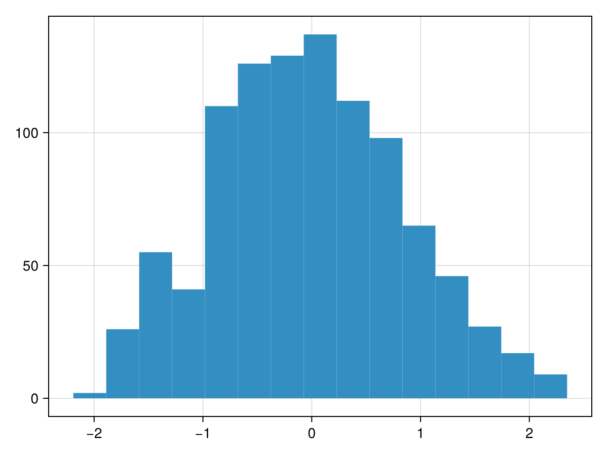

This is the trajectory of a walker at each step. The histogram above shows the number of these points in each bin.

# plotting trajectory
using CairoMakie
X = [r[1] for r in R]
Y = keys(X)
lines(X, Y)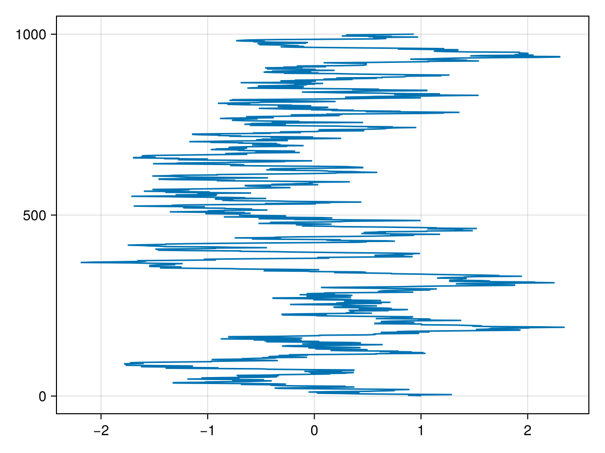

Using Distributions.jl

Here is an example of sampling the distribution functions in Distributions.jl.

# distribution
using Distributions
d = Normal(0, 1)

# sampling
using MetropolisAlgorithm
R = metropolis(x -> Distributions.pdf(d,x[1]), [1.0], n_steps=10000, d=1.0)

# reshape for plotting
X = [r[1] for r in R]
Y = keys(X)  .- 1

# figure
using CairoMakie
fig = Figure(
  size = (420,600),
  fontsize = 11,
  backgroundcolor = :transparent,
)

# histogram
axis = Axis(
  fig[1,1],
  limits = (-5, 5, 0, 1.1*Distributions.pdf(d,d.μ)),
  titlesize = 16.5,
  xlabelsize = 16.5,
  ylabelsize = 16.5,
  title = "Histogram",
  xlabel = "x",
  ylabel = "PDF(x)",
  backgroundcolor = :transparent,
)
hist!(axis, [first(r) for r in R], label = "Metropolis", bins = 50, normalization = :pdf)
lines!(axis, -50..50, x -> Distributions.pdf(d,x), label = "Exact", color=:black)
axislegend(axis, position = :rt, framevisible = false)

# trajectory
axis = Axis(
  fig[2,1],
  limits = (-5, 5, 0, length(R)),
  titlesize = 16.5,
  xlabelsize = 16.5,
  ylabelsize = 16.5,
  title = "Trajectory",
  xlabel = "x",
  ylabel = "steps",
  backgroundcolor = :transparent,
)
lines!(axis, X, Y, linewidth = 0.3, label = "Metropolis")
axislegend(axis, position = :rt, framevisible = false)

# display
fig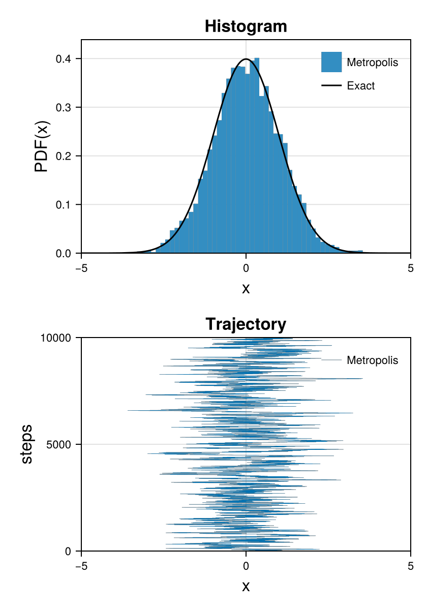

The output histograms are consistent with the input distribution functions.

# packages
using CairoMakie
using Distributions
using MetropolisAlgorithm

# initialize
fig = Figure(
  size = (1260,600),
  fontsize = 11,
  backgroundcolor = :transparent,
)

for n in 1:6

    # distribution
    d = [
        Normal(0, 1)
        SymTriangularDist(0, 1)
        Uniform(0, 1)
        Gamma(7.5, 1)
        TriangularDist(0, 1, 0.2)
        Semicircle(1)
    ][n]
    μ = Distributions.mean(d)
    σ = Distributions.std(d)

    # sampling
    R = metropolis(x -> Distributions.pdf(d,x[1]), [1.0], n_steps=100000, d=σ)

    # plot
    axis = Axis(
      fig[div(n-1,3)+1,rem(n-1,3)+1],
      limits = (-5*σ+μ, 5*σ+μ, 0, 1.2*maximum(Distributions.pdf(d,x) for x in -5*σ+μ:0.1:5*σ+μ)),
      titlesize = 16.5,
      xlabelsize = 16.5,
      ylabelsize = 16.5,
      title = "$d",
      xlabel = "x",
      ylabel = "PDF(x)",
      backgroundcolor = :transparent,
    )
    hist!(axis, [first(r) for r in R], label = "Metropolis", bins = 50, normalization = :pdf)
    lines!(axis, -50..50, x -> Distributions.pdf(d,x), label = "PDF", color=:black)
    axislegend(axis, position = :rt, framevisible = false)

end

fig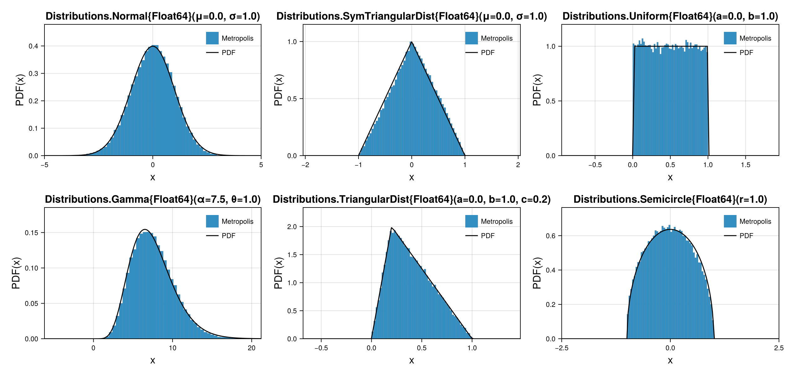

Minimal Working Example for Multiple-Walkers

Allocate memory by yourself for multiple walkers.

using MetropolisAlgorithm
p(x) = exp(-x[1]^2/2) / sqrt(2*π)
R = fill([0.0], 10000)

10000-element Vector{Vector{Float64}}:
 [0.0]
 [0.0]
 [0.0]
 [0.0]
 [0.0]
 [0.0]
 [0.0]
 [0.0]
 [0.0]
 [0.0]
 ⋮
 [0.0]
 [0.0]
 [0.0]
 [0.0]
 [0.0]
 [0.0]
 [0.0]
 [0.0]
 [0.0]

Each step is run without memory allocation for walkers, overwriting the second argument.

metropolis!(p, R)
R

10000-element Vector{Vector{Float64}}:
 [-0.36238507850531854]
 [-0.19199978354655345]
 [0.10116038096960867]
 [-0.15115420558082515]
 [0.23937914995383636]
 [0.2879693228773873]
 [-0.1918246338256846]
 [-0.3009792259374626]
 [0.31342363679799246]
 [-0.3442340774121988]
 ⋮
 [-0.33717019187073083]
 [-0.10952052900774756]
 [-0.0041925146814719705]
 [0.4620076789161992]
 [0.33793105410034685]
 [-0.17672256730925673]
 [-0.3587887732593451]
 [-0.07121928021019586]
 [-0.46588901882225797]

Use the For statement to repeat as many times as you like.

for i in 1:100
  metropolis!(p, R)
end
R

10000-element Vector{Vector{Float64}}:
 [-1.3735745632945977]
 [0.6428761697124191]
 [0.7376733732194536]
 [1.9735580246326685]
 [0.04731105571375638]
 [-0.32101146874912334]
 [0.8565757350576514]
 [-0.35705131512910027]
 [-0.09988536111317448]
 [-1.3407174022706663]
 ⋮
 [0.6861093924133987]
 [-0.453412478117208]
 [-0.34129270253490485]
 [-0.5565904506341147]
 [1.4263036204822108]
 [-0.13548063028507307]
 [1.3922958848536373]
 [1.8733985767517498]
 [0.15099900425304258]

Time evolution to reach equilibrium. The first several steps are not consistent with the correct distribution.

using MetropolisAlgorithm

# distribution function
p(x) = exp(-x[1]^2/2) / sqrt(2*π)

# figure
using CairoMakie
fig = Figure(size=(1680, 420))

# axis
axis1 = Axis(fig[1,1], limits=(-5, 5, 0, 1.1*p([0])), title="n=0")
axis2 = Axis(fig[1,2], limits=(-5, 5, 0, 1.1*p([0])), title="n=1")
axis3 = Axis(fig[1,3], limits=(-5, 5, 0, 1.1*p([0])), title="n=2")
axis4 = Axis(fig[1,4], limits=(-5, 5, 0, 1.1*p([0])), title="n=100")

# n = 0
R = fill(zeros(1), 10000)
hist!(axis1, [r[1] for r in R], bins=-5:0.1:5, normalization=:pdf)
lines!(axis1, -5..5, p, color=:black)

# n = 1
metropolis!(p, R)
hist!(axis2, [r[1] for r in R], bins=-5:0.1:5, normalization=:pdf)
lines!(axis2, -5..5, p, color=:black)

# n = 2
metropolis!(p, R)
hist!(axis3, [r[1] for r in R], bins=-5:0.1:5, normalization=:pdf)
lines!(axis3, -5..5, p, color=:black)

# n = 100
for i in 3:100
    metropolis!(p, R)
end
hist!(axis4, [r[1] for r in R], bins=-5:0.1:5, normalization=:pdf)
lines!(axis4, -5..5, p, color=:black)

# display
fig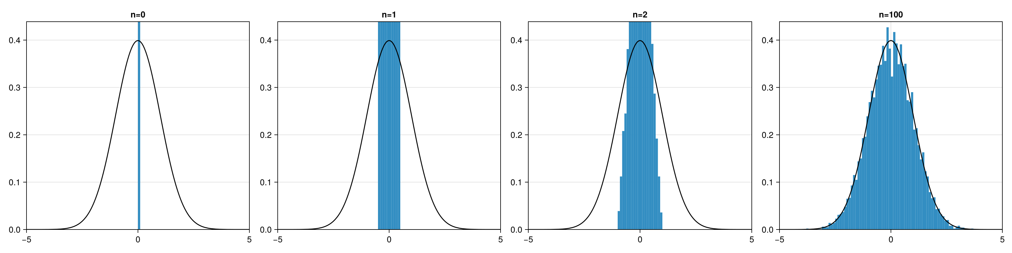

Three-dimensional Metropolis-walk

Here is an example of sampling a function like an atomic orbital (d-orbital).

Single-Walker

# sampling
using MetropolisAlgorithm
ψ(r) = r[1] * r[2] * exp(- r[1]^2 - r[2]^2 - r[3]^2)
p(r) = abs2(ψ(r))
R = metropolis(r -> abs2(ψ(r)), [1.0, 0.0, 0.0], n_steps=50000)

# plot
using CairoMakie
CairoMakie.activate!(type = "png")
fig = Figure(size=(420,420), figure_padding=0)
axis = Axis(fig[1,1], aspect=1, backgroundcolor=:black, limits=(-2,2,-2,2))
hidespines!(axis)
hidedecorations!(axis)
lines!(axis, [r[1] for r in R], [r[2] for r in R], linewidth=0.1, color="#00FFFF")
fig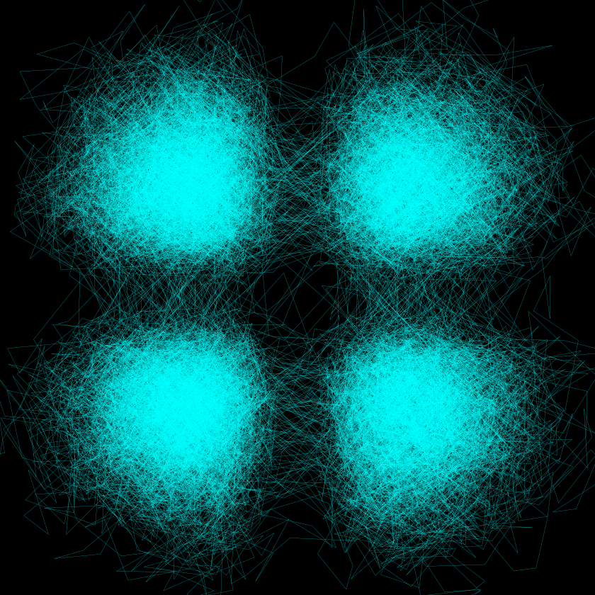

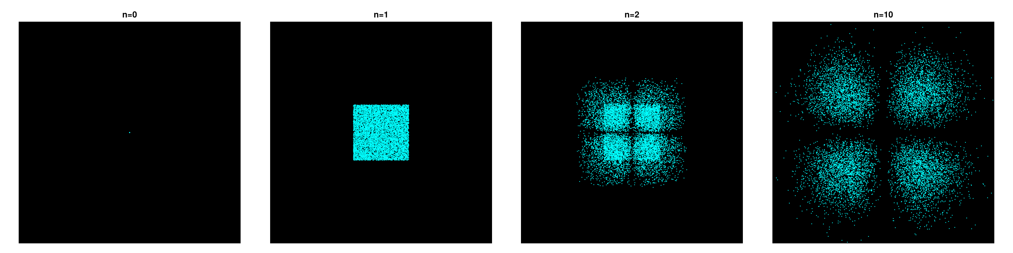
Multiple-Walkers

using MetropolisAlgorithm

# distribution function
ψ(r) = r[1] * r[2] * exp(- r[1]^2 - r[2]^2 - r[3]^2)
p(r) = abs2(ψ(r))

# figure
using CairoMakie
CairoMakie.activate!(type = "png")
fig = Figure(size=(1680, 420))

# axis
axis1 = Axis(fig[1,1], aspect=1, limits=(-2,2,-2,2), backgroundcolor=:black, title="n=0")
axis2 = Axis(fig[1,2], aspect=1, limits=(-2,2,-2,2), backgroundcolor=:black, title="n=1")
axis3 = Axis(fig[1,3], aspect=1, limits=(-2,2,-2,2), backgroundcolor=:black, title="n=2")
axis4 = Axis(fig[1,4], aspect=1, limits=(-2,2,-2,2), backgroundcolor=:black, title="n=10")
hidespines!(axis1)
hidespines!(axis2)
hidespines!(axis3)
hidespines!(axis4)
hidedecorations!(axis1)
hidedecorations!(axis2)
hidedecorations!(axis3)
hidedecorations!(axis4)

# n = 0
R = fill(zeros(3), 10000)
scatter!(axis1, [r[1] for r in R], [r[2] for r in R], markersize=2, color="#00FFFF")

# n = 1
metropolis!(p, R)
scatter!(axis2, [r[1] for r in R], [r[2] for r in R], markersize=2, color="#00FFFF")

# n = 2
metropolis!(p, R)
scatter!(axis3, [r[1] for r in R], [r[2] for r in R], markersize=2, color="#00FFFF")

# n = 10
for i in 1:10
    metropolis!(p, R)
end
scatter!(axis4, [r[1] for r in R], [r[2] for r in R], markersize=2, color="#00FFFF")

# display
fig